Ground-penetrating radar (GPR) was first patented in 1904 by Dr. Christian Hülsmeyer, a German scientist. It wasn’t until the 1970s, however, that GPR became a widely used tool for underground (or under-ice) surveying. Since then, it’s experienced widespread use in archaeology, utility detection, forensics and transportation, to name the most-common applications.
Few people realize that GPR has always been a 3D technology, assuming location is known (the X/Y coordinates). GPR’s primary purpose is to determine the Z coordinate, but GPR can be used to create a 3D point cloud—just like LiDAR.
Multiplicity Matters
Although GPR creates 3D coordinates, it does so on a very limited basis (unlike LiDAR). A single (successful) pass of a conventional GPR unit creates a single coordinate for (the top of) a given object or feature, using 2D imagery to display its location. This is due to the single pair of antennas employed: one transmitter and one receiver. This concept can be demonstrated by holding up a piece of paper sideways, as this is how much information is created. With just one antenna, it would take reams, cases and pallets of paper to render 3D underground data across large areas.
This is where signal multiplicity (i.e., antenna array) comes in. Only when taking a “GPR shot” of a given object from multiple angles can users create 3D positional data for that object. This concept was “borrowed” from paleontology when a utility contractor met a geophysicist using sound as the signal source (acoustic tomography). Dr. Alan Witten was using an array of geophones and a sawed-off shotgun to image dinosaur fossils for Oak Ridge National Labs in New Mexico. Witten Technologies was formed in 1994, and radar tomography (RT) was developed through the rest of the century, debuting in Manhattan after 9/11.
The first array was about two meters wide and contained 17 total antennas; 9 transmitters and 8 receivers in two parallel rows to create 16 discrete GPR channels. That’s not a magic number, as the total number of antennas in any given array can and does vary. Obviously, the width of the array dictates how much area is covered in one pass, and distance between the antennas creates the “3D” effect—more is better.
Placing Position
The other necessary component is geopositioning. If collecting (literally) thousands of images, users need to know exactly where every image is if they want to stitch them together on the back end. To do this, every antenna must be located with respect to its neighbors, and users have to know exactly where the array is as it moves across the earth.
To determine the position of the array while in motion, a robotic geodimeter total station can be used to track a prism pole mounted on the array. Interestingly, this is one way LiDAR and RT are identical, as both are “line-of-sight” dependent.
A trigger-wheel can also be used with controlled signal-firing frequency. Every four inches is adequate, but that isn’t a magic number. Forward speed dictates firing frequency, and a pace of roughly 2 mph is common. Even at that snail’s pace, you could do about half an acre per day. Like most technical components, velocity and data-collection rates have improved.
The other core component is software, which is employed in stages throughout the process. Specialized software governs the collection process, allowing the operator(s) to continuously monitor the process. On the backend, specialized software merges the imagery and geometry data to create a “data cube” from which utilities and other underground features are extracted and rendered in user-consumable form: typically via CAD software.
Getting to Deliverables
Deliverables are what matter to engineers, and this area has grown the quickest, given the now-pervasive concept of 3D geospatial CAD data. Although CAD previously wasn’t up to the task, 3D data could be produced with the help of a partner that used video gaming software.
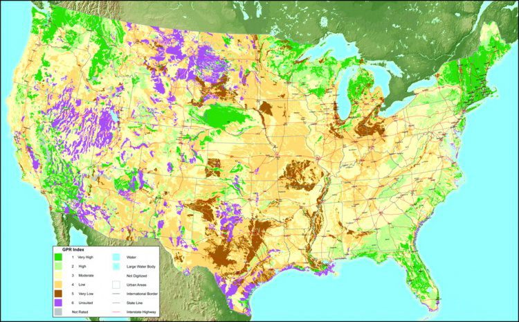
Unlike LiDAR, GPR presents more challenges than just “line-of-sight.” One is soil conductivity, in that conductive soils or other surface materials are GPR-opaque. They absorb the electromagnetic pulses, leaving no signal to return. There are places GPR works well, places it doesn’t work at all and many areas in-between. There’s actually a map for that.
Soil conductivity is a deciding factor on the effectiveness of GPR technology, and this map shows where suitable soils exist in the United States.
Assuming suitable soils, there’s also the matter of frequency. GPR operates within a specific radio-frequency range, where low frequencies penetrate further, but high frequencies are shallower and offer better resolution. Most arrays operate at a single frequency, although multiple (“step”)-frequency GPR arrays have recently been introduced. Now it’s possible to assess roadbed conditions while detecting utilities under the road.
Taking that a step further and (literally) bringing it all together, the recent marriage of above- and below-ground 3D sensing technologies make it possible to create a 3D image of reality. Pretty heavy, huh?
Andrew Lund, GISP, is a 20-year veteran of the utility mapping industry, with expertise in the separate but related fields of GIS, remote sensing, regulatory compliance, and 811 automation; e-mail: [email protected].


.jpg?width=225)